Cost-effectiveness analysis
This tutorial explains how to use the cost-effectiveness analysis tool presented in cea.
The tool calculates the costs, QALYs gained or any other label of one or multiple Universe instances.
Moreover, it is possible to use this tool for probabilistic sensitivity analysis (PSA) and univariate sensitivity analysis (USA) to incorporate uncertainty in cost and QALY estimates.
It can also find the (strongly or weakly) dominating Universe instances and plot them.
This allows simple post-processing of MISCore simulations.
We discuss:
How to write a data file to specify the costs/effects of each logged event or duration;
How to implement a regular CEA and find dominating strategies;
How to do a probabilistic sensitivity analysis;
How to do a univariate sensitivity analysis;
How to use implement different QALY values for age and sex groups.
Note
If you use built-in data for the costs and effects, you can skip the first part on the CEA data.
The starting point of any cost-effectiveness analysis is to have events and durations results from which you can calculate costs and benefits of a given scenario. As an example, you may use the following model run in which we compare a scenario of screening for endometrial cancer with a non-screening scenario. You may run it yourself to obtain the dataframes used in the examples.
Show/hide full code
 1import pandas as pd
 2
 3from miscore import Model, processes, Universe
 4from miscore.tools import cea
 5from miscore.tools.cea.data import population_norms
 6
 7# Birth process
 8birth = processes.Birth(
 9    name="birth",
10    year=1975
11)
12
13# OC process
14oc = processes.OC(
15    name="oc",
16    life_table=processes.oc.data.us_2009.life_table,
17)
18
19# EC process
20ec = processes.EC.from_data(processes.ec.data.us)
21
22# EC screening process
23ec_screening = processes.EC_screening.from_data(processes.ec_screening.data.example)
24
25# Universes
26no_screening = Universe(
27    name="no_screening",
28    processes=[
29        birth,
30        oc,
31        ec
32    ]
33)
34
35screening = Universe(
36    name="screening",
37    processes=[
38        birth,
39        oc,
40        ec,
41        ec_screening
42    ]
43)
44
45# Model
46model = Model(
47    universes=[
48        no_screening,
49        screening
50    ]
51)
52
53# Run model
54result = model.run(
55    n=1e5,
56    seed=123,
57    event_ages=range(0, 101, 1),
58    duration_ages=range(0, 101, 1),
59    event_years=range(1975, 2075, 1),
60    duration_years=range(1975, 2075, 1),
61    verbose=True
62)
The complete code used in this tutorial is shown at the bottom of this page,
you may also download the .py file cea_example_run.py.
Data file
In order to calculate the costs/effects of strategies, they must be specified in a data file. A data file consists of up to three elements (one of them is optional).
Labels
The post-processing code allows to calculate multiple quantities.
For example the costs, the (Quality-Adjusted) Life-Years (QALY/LY) or the number of hysterectomies in each Universe.
The name of each labels to be measured has to be specified in the parameter labels in a list.
65labels = ("costs", "LY", "QALY", "n_hysterectomies")
Discount rates (optional)
The data can be discounted (as will be discussed later in this tutorial). It is possible to either specify one discount rate for all quantities or specify separate rates for each label. In the latter case, the rates have to be specified in the data file with a list:
66discount_rates = (0.03, 0.03, 0.03, 0.00)
Note that the order of the rates must correspond with the order in labels.
If the discount rate is the same for all quantities, discount_rates can simply be a floating point number.
Costs and effects data
In the data file, costs and effects should be specified for tags that are logged in the events, durations and snapshots tables.
The costs/effects for a tag are specified in one or multiple data sets.
The use of multiple datasets in the costs and effects specification allows varying costs and utilities by subpopulation.
Each data set is a dictionary within the dictionary ce which consists of up to five
elements: conditions, durations, events, snapshot_years and snapshot_ages.
We will discuss the following example:
68# We declare a cost-effectiveness dataset, associating tags of interest with benefits and harms.
69# The dataset consists of two parts: lifelong costs/utilities and utilities for women aged 45-.
70cea_data = {
71    "Lifelong": {
72        "conditions": [],
73        "durations": {
74            # Total number of Life Years
75            "life": (0, 1, 1, 0),
76        },
77
78        "events": {
79            # Costs of treatment
80            "ec_clinical": (35763, 0, 0, 1),
81            "ec_screening_hysterectomy": (15276, 0, 0, 1),
82
83            # Count number of deaths in population
84            ".*death": "deaths"
85        },
86    },
87    "Menopause": {
88        "conditions": [("age", "<", 45)],
89        "durations": {
90            # Disutilities due to surgically induced menopause
91            ("ec_clinical_month1", "ec_screening_hysterectomy_month1"): (0, 0, -0.44, 0),
92            ("ec_clinical_months2-3", "ec_screening_hysterectomy_months2-3"): (0, 0, -0.26, 0),
93            ("ec_clinical_cont", "ec_screening_hysterectomy_cont"): (0, 0, -0.12, 0),
94        },
95        "events": {}
96    },
97}
Conditions
These cost-effectiveness data consist of two parts: Lifelong and Menopause.
The Lifelong part does not have any conditions.
The Menopause part, however, only applies for events and durations that occurred before age 45.
This part contains disutilities (i.e. negative QALYs) caused by surgically induced menopause.
Since women aged under 45 likely had not had their menopause yet, these disutilities only apply to events and durations before age 45.
Note
It is allowed to specify multiple conditions in conditions, for example
"conditions": [("universe", "==", "screening"), ("age", "<", 65), ("year", ">=", 1993)]
would only apply to people in the Universe screening that were younger than 65 in the years after 1993.
Conditions can be applied to any column in the durations and events tables (including stratum, cohort, year, age and Universe).
The feasible operators are <, <=, ==, !=, >=, >.
Durations and events
Next, both parts specify costs and utility data for various events and duration tags.
For example, the Lifelong part specifies that an occurrence of the life tag in the durations yields 0 costs, 1 QALY, 1 LY and 0 hysterectomies.
This represents the total number of lifeyears of individuals.
Lifelong also specifies the costs of treatment and hysterectomies.
The event tags ec_clinical and ec_screening_hysterectomy are associated with costs and with 1 hysterectomy.
No (reduction in) lifeyears and QALYs are associated with these tags, however.
Finally, the Lifelong part counts the total number of deaths.
By specifying a string instead of a tuple of values, the specified tags are aggregated and counted, without multiplying by costs or utility values.
As a result, an extra label deaths will be added to the outputs.
Note that we used .*death, which means “all tags that end with ‘death’”.
This is an example of regex.
Their documentation will show more examples of regex rules.
The Menopause part only specifies disutilities for six duration tags.
The first month of surgically induced menopause leads to a 0.44 reduction in yearly QALYs (so effectively a 0.04 QALY reduction).
The second and third month lead to a 0.26 reduction in yearly QALYs.
After that, there is a 0.12 reduction in yearly QALYs, until the age of 45.
Note that these disutilities are the same for hysterectomies due to clinical diagnosis and due to screening.
By setting two or more tags within a tuple (in brackets), the same cost/effect values can be assigned to these tags.
Note
In general, the value for QALYs are negative for all tags except “life”.
Note
In this example, costs/effects are specified for durations and events only.
In a similar way, costs/effects can also be specified for snapshot_years and snapshot_ages.
Note
It is also possible to specify the disutilities of surgically induced menopause using regex.
The following would yield the same results.
Note, however, that the use_regex parameter in the cost_effectiveness_analysis() function should be set to True.
# Disutilities due to surgically induced menopause
"ec_.*_month1": (0, 0, -0.44, 0),
"ec_.*_months2-3": (0, 0, -0.26, 0),
"ec_.*_cont": (0, 0, -0.12, 0),
Functions in the cost-effectiveness analysis module
The cost-effectiveness analysis module contains four functions which are discussed in this section.
They require the events and durations output from the simulation run as inputs.
If the simulation was run in the same script, they can be retrieved from the Result object as follows:
 99# Retrieve the events and durations tables obtained by simulation
100durations = result.durations
101events = result.events
Alternatively, in case the durations and events output were generated by another script, the .csv or .pkl output files can be imported as follows.
import pandas as pd

# Import the (concatenated) events and durations tables obtained by simulation
durations = pd.read_csv("durations.csv")
events = pd.read_csv("events.csv")
import pickle

# Import the (concatenated) events and durations tables obtained by simulation
durations = pickle.load(open('durations.pkl','rb'))
events = pickle.load(open('events.pkl','rb'))
Note
The cost-effectiveness module takes only one events and one durations table as an input.
These should contain the durations and events of each Universe you want to evaluate.
Therefore, if your simulation was done with more than one Model, make sure to concatenate all events and durations to one table respectively.
You can do so by adding all events/durations to two separate lists and using the concat() function to concatenate all events/durations dataframes:
# If the simulation was done with three models, there are three Result instances.
# First put all events and durations dataframes in separate lists
events_list = [result1.events, result2.events, result3.events]
durations_list = [result1.durations, result2.durations, result3.durations]

# Then concatenate the lists of events and durations into one dataframe
events = pd.concat(events_list)
durations = pd.concat(durations_list)
This note can be ignored if your simulation used multiple Universe instances instead of multiple Model runs.
Calculate costs and effects
The cost_effectiveness_analysis() function calculates the costs and effects for the different simulated Universe instances.
It can be used as follows:
103ce_result = cea.cost_effectiveness_analysis(durations=durations,
104                                            events=events,
105                                            cea_data=cea_data,
106                                            cea_labels=labels,
107                                            division_factor=100000,
108                                            discount_by="age",
109                                            discount_start=40,
110                                            discount_rate=discount_rates,
111                                            group_by=["universe"],
112                                            use_regex=True,
113                                            verbose=True
114                                            )
The ce_result object is a CEAResult instance as the output.
The CEAResult page shows the elements included in this class.
The most relevant result is ce.cea_output, which contains outcomes by type of outcome and Universe.
Printing these outcomes will show the table of cost-effectiveness outputs.
116print(ce_result.cea_output)
id |
universe |
label |
number |
|---|---|---|---|
0 |
no_screening |
costs |
8289.900573 |
1 |
no_screening |
LY |
60.960182 |
2 |
no_screening |
QALY |
60.898495 |
3 |
no_screening |
nr_hysterectomy |
0.359300 |
4 |
no_screening |
deaths |
1.000000 |
5 |
screening |
costs |
15376.644948 |
6 |
screening |
LY |
61.111235 |
7 |
screening |
QALY |
60.211758 |
8 |
screening |
nr_hysterectomy |
0.853680 |
9 |
screening |
deaths |
1.000000 |
The cost_effectiveness_analysis() function requires the following parameters:
cea_dataandcea_labelsshould be used to specify the cea input data (cea_dataandlabels) from the data file.Simulation output, such as the
durationsandeventstables that were generated by the simulation, and/or thesnapshots_agesandsnapshots_yearsdataframes should be specified. Alternatively, the entireresultobject can be supplied, from which the output dataframes will be harvested.
Additionally, the function has a large variety of optional parameters.
Outcomes can be discounted by age or year by setting
discount_byto either “year” or “age”. This also requires setting a first year/age to start discounting asdiscount_start, as well as adiscount_rate, which may either be a single floating point rate or an iterable with a rate for each of the outcomes incea_labels.division_factorscales the CEA results by dividing all outcomes by the specified factor. For instance, to get results per individual alive at the start of simulation, specify the population sizenof your simulation. Alternatively, to scale to a given number of individuals alive at the start of simulation, usendivided by the scale. For example if you want to report result per 1,000 individuals.Next, it is possible to set a reference value for each of the quantities. Then the costs/effects of all other universes are calculated with respect to the reference
Universe, i.e. the costs/effects of the reference are subtracted from each otherUniverse. It can be specified either by a name of aUniversein the durations/events tables or by a tuple with explicit values. For example the following two specifications would give the same result:118# Now we include a reference strategy. There are two methods: 119reference_strategy = (8289.90057, 60.96018, 60.89849, 0.35930, 1.0) 120reference_strategy = "no_screening" 121 122ce_result = cea.cost_effectiveness_analysis(durations=durations, 123 events=events, 124 cea_data=cea_data, 125 cea_labels=labels, 126 division_factor=1000000, 127 discount_by="age", 128 discount_start=40, 129 discount_rate=discount_rates, 130 group_by=["universe"], 131 use_regex=True, 132 reference=reference_strategy 133 ) 134 135print(ce_result.cea_output)
id
universe
label
number
5
screening
costs
708.674438
6
screening
LY
0.015105
7
screening
QALY
-0.068674
8
screening
n_hysterectomies
0.049438
Note
If the reference values are specified by a tuple, the values must match the scale per
division_factor.Costs and utilities can be grouped by variables other than
Universeby specifying thegroup_byparameter. The following example will show the costs and effects perUniverseand per year. The outcomes can be grouped by universe, cohort, stratum, year and tag (the labels of events and durations), and any of their combinations.137# Now we group the results by universe and year only. 138group_by = ["universe", "year"] 139ce_result = cea.cost_effectiveness_analysis(durations=durations, 140 events=events, 141 cea_data=cea_data, 142 cea_labels=labels, 143 division_factor=1000000, 144 discount_by="age", 145 discount_start=40, 146 discount_rate=discount_rates, 147 group_by=group_by, 148 use_regex=True) 149print(ce_result.cea_output)
id
universe
year
label
number
1
no_screening
0.0
LY
0.099671
2
no_screening
0.0
QALY
0.099671
4
no_screening
0.0
deaths
0.000649
5
no_screening
1.0
costs
0.178815
6
no_screening
1.0
LY
0.099331
…
…
…
…
…
1001
screening
99.0
LY
0.000386
1002
screening
99.0
QALY
0.000386
1003
screening
99.0
n_hysterectomies
0.000005
1004
screening
99.0
deaths
0.000819
1009
screening
100.0
deaths
0.001797
The boolean
verbose, set to True by default, will warn you of any tags that were in the simulation results but were not included in thecea_datadictionary. It will also communicate the progress of the cost effectiveness analysis.For the events, durations and snapshots tables separately, two types of tags are printed. First, unused tags are those that are specified in the data file, but are not used in the durations/events tables. Second, unspecified tags are those that are not specified in the data file, but are used in the durations/events tables. This option is useful when generating a new data file, however it also takes extra running time. Even though the option defaults to
True, it is advised to turn it toFalsein final runs.Note
When you use regex to associate tags with outcomes and effects, make sure you set the option
use_regextoTrue!
Finding dominating universes
The dataframe that results from cost_effectiveness_analysis() contains the costs and effects of each Universe.
If each Universe is generated with different screening strategies, one may be interested in the dominating Universe set.
The functions find_pareto() and find_efficient() find the strongly and weakly dominating universes respectively.
The functions expect that you have somewhat transformed your ce.cea_output data, with the labels of your
outcomes as columns. We can easily get such a table by using the pandas.pivot_table function. This has the
added benefit that we can specify fill_value=0 to fill in any outcomes that do not occurr for each Universe:
152# Pivot results by universe to search for efficient universes
153universe_table = pd.pivot_table(ce_result.cea_output, aggfunc="sum",
154                                columns="label", values="number", index="universe")
155print(universe_table)
Note
pd.pivot_table by default calculates the mean across the index values (in this case the different Universe instances,
supply aggfunc=”sum” to get the sum of all values in the number column.
This gives us the right type of table:
universe |
costs |
LY |
QALY |
nr_hysterectomy |
deaths |
|---|---|---|---|---|---|
no_screening |
828.990057 |
6.096018 |
6.089849 |
0.035930 |
0.1 |
screening |
1537.664495 |
6.111124 |
6.021176 |
0.085368 |
0.1 |
We can then supply this table to our functions that determine the efficiency frontiers, containing each efficient Universe.
156# Here we search for the dominating strategies
157dominating_strategies = cea.find_pareto(universe_table)
158efficient_strategies = cea.find_efficient(universe_table)
159print(efficient_strategies)
universe |
costs |
LY |
QALY |
nr_hysterectomy |
deaths |
icer |
|---|---|---|---|---|---|---|
no_screening |
828.990057 |
6.096018 |
6.089849 |
0.03593 |
0.1 |
-inf |
Note
By default, the functions search for the Universe instances that minimise the costs and maximise the QALYs.
However, users may alter these choices by specifying costs_label and effects_label respectively.
For example, Universe instances that minimise the number of hysterectomies and maximise the LY are found by
dominating_strategies = find_pareto(universe_table, costs_label="nr_hysterectomy", effects_label="LY")
Note
The find_efficient() function also has a near_efficiency_margin parameter.
This parameter takes a number between 0 and 1.
Strategies of which the effects_label is within near_efficiency_margin * 100% of the frontier are considered near-efficient and included in the frontier.
efficient_strategies = find_pareto(universe_table, near_efficiency_margin=0.02)
Note
If you performed a PSA as part of your cost effectiveness analysis, you may be interested in the efficient
frontier and the ICERs for each of the random draws. This allows you to estimate the probability per your
stochastic sensitivity analysis of your strategy being on the frontier, as well as the probability that
your ICER is below a given threshold. The find_efficient() function will automatically
recognize that you have output from a PSA, if you have grouped your cea_output by both Universe and
psa_set, with psa_set as the first index level:
psa_table = pd.pivot_table(ce.cea_output, columns="label", values="number", index=["psa_set", "universe"])
dominating_strategies_psa = find_pareto(universe_table)
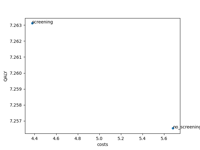
Scatter plot of universes
Finally it is possible to make a scatter plot of the costs and effects of the calculated Universe with:
161# The scatter_ce function allows us to plot the universes on the cost-QALY plane
162cea.scatter_ce(universe_table, x_label="costs", y_label="QALY", tags="index")
163cea.show()
This code generates a scatter plot showing the costs of each Universe on the horizontal axis and QALYs on the vertical axis.
Note that it is possible to vary the quantities on each of the axes with the parameters x_label and y_label.
Additionally, it is possible to show a string with each scatter dot in the graph by specifying the parameter tags.
The value index will add the value of the index of the specified DataFrame to the dot (usually this is the name of the Universe).
The value number will assign a number to each of the dots, this may improve the readability.
Finally, the function takes kwargs that are passed to matplotlib, allowing the plots to be styled.
The figure below shows the result. Note that in your analysis the plane may be populated by more Universe outcomes than
only the two generated by our example run.
Probabilistic Sensitivity Analysis (PSA)
In the above examples, costs and effects were specified as a single value. However, sometimes it can be useful to perform sensitivity analyses on costs and effects of one or multiple tags. For that, you can specify a probability distribution in place of the single value in the input dictionary:
165# Next, we do an example of a probabilistic sensitivity analysis
166labels = ["costs", "LY", "QALY", "n_hysterectomy"]
167discount_rates = (0.03, 0.01, 0.01, 0.00)
168
169# PSA-like input
170# We declare a cost-effectiveness dataset, associating tags of interest with costs and effects
171psa_data = {
172    "Lifelong": {
173        "conditions": [],
174        "durations": {
175            # Total number of Life Years
176            "life": (0, 1, (1, 0.8) * 1000, 0),
177        },
178        "events": {
179            # Costs of treatment
180            "ec_clinical": (("norm", {"loc": 35763, "scale": 5960}), 0, 0, 1),
181            "ec_screening_hysterectomy": (("norm", {"loc": 15276, "scale": 2546}), 0, 0, 1),
182
183            # Count number of deaths in population
184            ".*death": "deaths"
185        },
186    },
187    "Menopause": {
188        "conditions": [("age", "<", 45)],
189        "durations": {
190            # Disutilities due to surgically induced menopause
191            ("ec_clinical_month1", "ec_screening_hysterectomy_month1"): (0, 0, -0.44, 0),
192            ("ec_clinical_months2-3", "ec_screening_hysterectomy_months2-3"): (0, 0, -0.26, 0),
193            ("ec_clinical_cont", "ec_screening_hysterectomy_cont"):
194                (0, 0, ("uniform", {"loc": -0.12, "scale": 0.10}), 0),
195        },
196        "events": {}
197    },
198}
In this example, the disutilities for the durations ec_clinical_month1 and ec_screening_hysterectomy_month1 follow a normal
distribution with mean -0.44 and standard deviation 0.05.
Disutilities of ec_clinical_month23 and ec_screening_hysterectomy_month23 follow a uniform distribution with
lowerbound -0.39 and upperbound 0.13.
Any distribution available in scipy.stats can be used.
All distributions and their parameters are listed
here.
Another option is to specify a tuple of possible values for costs and effects as a user.
An example of this is shown for event tag ec_clinical_cont and ec_screening_hysterectomy_cont.
Disutilities for these durations alternate between -0.16 and 0.08.
Note
For larger analyses, like a PSA, efficiency is essential. To speed up your run, consider removing any unnecessary tags from the events dataframe before using it in your PSA.
We then need to tailor our inputs to the cost_effectiveness_analysis() function to perform a Probabilistic Sensitivity Analysis (PSA). To do so, set the parameter psa_n_samples to the desired number
of draws from the distributions defined for each of the inputs. When there are user-supplied values for each of the draws (i.e. an array of a given
length n was supplied to perform the PSA), make sure psa_n_samples matches the length of the user-supplied draws. To
make sure your PSA draws are reproducible, set a value for psa_seed.
200# Calculate costs and effects for each PSA draw
201ce_result = cea.cost_effectiveness_analysis(result=result,
202                                            cea_data=psa_data, cea_labels=labels,
203                                            division_factor=1e5, discount_by="age",
204                                            discount_start=40,
205                                            discount_rate=discount_rates,
206                                            group_by=["universe"],
207                                            psa_n_samples=2000,
208                                            psa_seed=42195)
209print(ce_result.cea_output)
We are now returned a result DataFrame with separate outputs by label and Universe for each of the possible
parameter draws out of the 2000 we simulated. The distribution of your outputs across these draws should inform you
of the uncertainty surrounding your initial estimate.
id |
universe |
psa_set |
label |
number |
|---|---|---|---|---|
0 |
no_screening |
0 |
costs |
8171.210975 |
1 |
no_screening |
0 |
LY |
69.894512 |
2 |
no_screening |
0 |
QALY |
69.846467 |
3 |
no_screening |
0 |
n_hysterectomy |
0.359300 |
5 |
no_screening |
1 |
costs |
7501.383817 |
… |
… |
… |
… |
… |
19993 |
screening |
1998 |
n_hysterectomy |
0.853680 |
19995 |
screening |
1999 |
costs |
13180.019709 |
19996 |
screening |
1999 |
LY |
70.150378 |
19997 |
screening |
1999 |
QALY |
55.839194 |
19998 |
screening |
1999 |
n_hysterectomy |
0.853680 |
Note
The option of performing a PSA also allows for different outputs to be included in the CEAResult object.
Setting return_psa_seeds to True, the seeds for each of the different inputs are returned. The user-supplied
seed is used to generate these seeds, to ensure that each input always starts the draw from the same point in the random number stream.
Setting return_psa_values to True, will return a DataFrame object with the exact values for each PSA draw and input tag. This
can be valuable in plotting the relationship between your aggregated outcomes for each draw, and the values of the inputs in each of these draws.
Depending on the number of inputs used and the value of psa_n_samples, this may be a memory-intensive DataFrame object.
Setting return_descriptives to True, will return a DataFrame object with descriptive sample statistics of each of the
inputs, across all of the PSA draws. This may be valuable in evaluating whether the specified distribution for an
input is resulting in the intended sample distribution, and whether psa_n_samples is sufficient to reduce the discrepancy
between the sample distribution and the intended distribution.
Univariate Sensitivity Analysis (USA)
Alternatively, you may be interested in the effect of individual inputs, changed one at a time. To this end,
the same dataset used for performing the PSA may be used for conducting a Univariate Sensitivity Analysis (USA).
To do so, set perform_usa to True. Rather than drawing all the values simultaneously, every draw will only have
one value changed at a time. In the DataFrame CEAResult.usa_values, you can find which value was changed to which input
for each of the usa_set values in CEAResult.cea_output.
By default, the values are each set at their 2.5%, 5%, 25%, 50%, 75%, 95% and 97.5% percentile values, per the distribution
used for the PSA. For PSA inputs for which a list of n values was supplied, the sample quantile values are used.
The quantiles used can be specified with the argument usa_quantiles if needed.
An example of performing a Univariate Sensitivity Analysis is given below.
211# Alternatively, we may perform a Univariate Sensitivity Analysis, in which values
212# are changed one by one.
213ce_result = cea.cost_effectiveness_analysis(result=result,
214                                            cea_data=psa_data, cea_labels=labels,
215                                            division_factor=1e5, discount_by="age",
216                                            discount_start=40,
217                                            discount_rate=discount_rates,
218                                            reference="no_screening",
219                                            group_by=["universe"],
220                                            perform_usa=True)
221# The output is now grouped by `usa_set` rather than `psa_set`
222print(ce_result.cea_output)
223
224# The `usa_values` DataFrame shows which input corresponds to which `usa_set`
225print(ce_result.usa_values)
Show full output
The output is now given by:
idx |
universe |
usa_set |
label |
number |
|---|---|---|---|---|
140 |
screening |
0 |
costs |
6624.022297 |
141 |
screening |
0 |
LY |
0.255866 |
142 |
screening |
0 |
QALY |
-0.283104 |
143 |
screening |
0 |
n_hysterectomy |
0.494380 |
145 |
screening |
1 |
costs |
6698.415765 |
… |
… |
… |
… |
… |
273 |
screening |
26 |
n_hysterectomy |
0.494380 |
275 |
screening |
27 |
costs |
7086.744375 |
276 |
screening |
27 |
LY |
0.255866 |
277 |
screening |
27 |
QALY |
-0.602420 |
278 |
screening |
27 |
n_hysterectomy |
0.494380 |
Specified by the usa_values DataFrame, where it is specified which input
is set to which value (corresponding to a particular quantile of its distribution)
to generate the input related to the usa_set index:
id |
usa_ceaset |
usa_table |
usa_tag |
usa_label |
usa_value |
usa_quantile |
|---|---|---|---|---|---|---|
0 |
Lifelong |
events |
ec_clinical |
costs |
47444.385348 |
0.025 |
1 |
Lifelong |
events |
ec_clinical |
costs |
45566.327617 |
0.050 |
2 |
Lifelong |
events |
ec_clinical |
costs |
39782.958911 |
0.250 |
3 |
Lifelong |
events |
ec_clinical |
costs |
35763.000000 |
0.500 |
4 |
Lifelong |
events |
ec_clinical |
costs |
31743.041089 |
0.750 |
5 |
Lifelong |
events |
ec_clinical |
costs |
25959.672383 |
0.950 |
6 |
Lifelong |
events |
ec_clinical |
costs |
24081.614652 |
0.975 |
7 |
Lifelong |
events |
ec_screening_hysterectomy |
costs |
20266.068305 |
0.025 |
8 |
Lifelong |
events |
ec_screening_hysterectomy |
costs |
19463.797334 |
0.050 |
9 |
Lifelong |
events |
ec_screening_hysterectomy |
costs |
16993.250904 |
0.250 |
10 |
Lifelong |
events |
ec_screening_hysterectomy |
costs |
15276.000000 |
0.500 |
11 |
Lifelong |
events |
ec_screening_hysterectomy |
costs |
13558.749096 |
0.750 |
12 |
Lifelong |
events |
ec_screening_hysterectomy |
costs |
11088.202666 |
0.950 |
13 |
Lifelong |
events |
ec_screening_hysterectomy |
costs |
10285.931695 |
0.975 |
14 |
Lifelong |
durations |
life |
QALY |
0.800000 |
0.025 |
15 |
Lifelong |
durations |
life |
QALY |
0.800000 |
0.050 |
16 |
Lifelong |
durations |
life |
QALY |
0.800000 |
0.250 |
17 |
Lifelong |
durations |
life |
QALY |
0.900000 |
0.500 |
18 |
Lifelong |
durations |
life |
QALY |
1.000000 |
0.750 |
19 |
Lifelong |
durations |
life |
QALY |
1.000000 |
0.950 |
20 |
Lifelong |
durations |
life |
QALY |
1.000000 |
0.975 |
21 |
Menopause |
durations |
(ec_clinical_cont, ec_screening_hysterectomy_cont) |
QALY |
-0.022500 |
0.025 |
22 |
Menopause |
durations |
(ec_clinical_cont, ec_screening_hysterectomy_cont) |
QALY |
-0.025000 |
0.050 |
23 |
Menopause |
durations |
(ec_clinical_cont, ec_screening_hysterectomy_cont) |
QALY |
-0.045000 |
0.250 |
24 |
Menopause |
durations |
(ec_clinical_cont, ec_screening_hysterectomy_cont) |
QALY |
-0.070000 |
0.500 |
25 |
Menopause |
durations |
(ec_clinical_cont, ec_screening_hysterectomy_cont) |
QALY |
-0.095000 |
0.750 |
26 |
Menopause |
durations |
(ec_clinical_cont, ec_screening_hysterectomy_cont) |
QALY |
-0.115000 |
0.950 |
27 |
Menopause |
durations |
(ec_clinical_cont, ec_screening_hysterectomy_cont) |
QALY |
-0.117500 |
0.975 |
Using population reference QALY values for different age- and sex groups
In performing cost-effectiveness analyses, it can often be easy to set decrements for health utility
for the particular health states we are simulating, and to set the QALY value for our "life" tag to 1.0.
This approach, however, assumes that anyone not experiencing the specific health state, is in perfect health.
Especially in older populations, other morbidities are very likely to influence the general level of health utility,
causing the average QALY value to never be as high as 1.0. Even younger populations often have an average
health utility level around 0.90.
It is therefore crucial to adjust the population reference values for any cost-effectiveness
analysis. This could be done by adjusting the "life" tag QALY value to some value below 1.0, but we
also include a tool for doing this separately for each age category. For this, the data module
includes the population_norms module with the add_population_norms() function, which adjusts
your cost-effectiveness input dictionary for the average population health utility, by age and sex.
Population norm utilities can be supplied by the user as a dataframe, or can be taken from the internally stored
values from the literature for the US, the UK, NL or CH.
In this example, the add_population_norms() function uses the internally stored population norm values
for the Dutch population. We can view this data by importing the dataset only.
from miscore.tools.cea.data.population_norms import data
data[(data.Country=="nl") & (data.Sex=="total") & (data.Method=="EQ5D")].head()
Country |
Agemin |
Agemax |
Yearmin |
Yearmax |
Sex |
Utility |
SE |
Method |
|---|---|---|---|---|---|---|---|---|
nl |
0 |
25 |
0 |
2200 |
total |
0.938 |
0.021 |
EQ5D |
nl |
25 |
35 |
0 |
2200 |
total |
0.910 |
0.012 |
EQ5D |
nl |
35 |
45 |
0 |
2200 |
total |
0.922 |
0.013 |
EQ5D |
nl |
45 |
55 |
0 |
2200 |
total |
0.874 |
0.019 |
EQ5D |
nl |
55 |
65 |
0 |
2200 |
total |
0.869 |
0.027 |
EQ5D |
Note
The method by which the utilities are derived in the literature may also differ, this is what the Method
column reports. For most countries, Visual Analogue Scale (VAS) values are included, as well as values derived
by means of population valuations of the EQ-5D survey. Although the EQ-5D is the most commonly used method, it
may be valuable to your research to perform a sensitivity analysis in which results with both value sets are compared.
Note
Yearmin and Yearmax columns are included, which may report any conditions on the calendar year for
which to apply the population health utilities. It could be that survey values were used which are
updated over the years, such that separate calendar years are associated with new population health
utility values. For the current internally included values, these limits are set to 0 and 2200, since
only one survey year is used.
An example call of the add_population_norms() function is given below.
We see that we supplied a CEA dataset called ce to this function.
For each age category, new entries in ce are created in which the life QALY value, and any other disutility values is adjusted.
These values which were previously relative to a health utility value of 1, are now set to be relative to the population norm utility.
The adjustment of disutility values depends on the disutility_method parameter. The available methods are:
"proportional":Disutilities are adjusted proportionally to the difference between the original
lifeutility (set to 1.0) and the population norm utility. Hence, for individuals ages 0 to 25, the disutility forec_clinicalchanges from-0.1to-0.0938.
"nominal":Disutilities are adjusted by the absolute difference between the
lifeutility and the population norm utility. Now for individuals ages 0 to 25, the disutility forec_clinicalchanges from-0.1to-0.038. Because the adjusted disutility depends on the duration of the disutility, it is not possible to change event disutilities using this method.
"nominal_censored":Similar to the
"nominal"method, but the disutility values are capped at the population norm utility level. This ensures that the simulated disease state does not result in a better health utility than the general population for individuals of the same age. Before using this method, it should be carefully considered whether your diseased population could be healthier than the average individual of the same age. Also similar to the"nominal"method, it is not possible to change event disutilities using this method.
Here is how you might use the add_population_norms() function with these adjustments:
Note that the inputs in the new ce dictionary are stored with tuple indexes (a, b), where a is the name of the input dataset, in this case 'x', and
b is the row index in the dataframe of population norm utilities.
227# Optionally correct our cost-effectiveness input data for population norm values
228cea_data['Lifelong']['durations']['ec_clinical'] = (0, 0, -0.1, 0)
229ce_input = population_norms.add_population_norms(
230    data_quantities=cea_data,
231    country="nl",
232    sex="total",
233    data_labels=processes.ec_screening.data.cea.labels,
234    disutility_tags=['ec_clinical'],
235    disutility_method="nominal"
236)
237print(ce_input[('Lifelong', 63)]['conditions'])
238print(ce_input[('Lifelong', 63)]['durations'])
[('age', '>=', 0), ('age', '<', 25)]
{'life': (0, 1, 0.938, 0), 'ec_clinical': (0, 0, -0.03799999999999995, 0)}
If you would like the health disutilities to be taken relative to whatever the reference health utility is, simply leave
the argument disutility_tags blank to prevent any disutilities from being changed.
It is also possible to supply your own population norm utility values. To do so, use the argument
norm_data. Make sure the input is a pandas DataFrame which includes all the columns shown in the
example above.
Note
We include also the SE column, which contains standard errors of the health utility values. These may be used
in order to generate Univariate or Probabilistic Sensitivity Analysis cea sets.
To generate an adjusted cea dataset that can be used in a Probabilistic Sensitivity Analysis, simply
set the argument n_psa_draws to the same n that you will use for your PSA. Normally distributed
norm utility values will be drawn, per the standard error in the SE column. The resulting dataset
may simply be passed on to cost_effectiveness_analysis, and for each of the n draws the corresponding
norm utility will be used. The disutility values for all disutility_tags will be adjusted so as to
preserve the same overall utility in the disease-specific state (i.e. if the random draw results in a decrease
of the norm utility by 0.1, the disutility will be adjusted by 0.1 to yield the same nominal disease-specific utility).
You may simultaneously generate random draws for the disutility tags. To do so, simply specify a distribution
for the disutility value as you would for any other PSA input. If a disutility tag is present but no distribution
is given, a constant nominal health-specific utility will be assumed (i.e. the sum of the norm utility and the disutility
will be held constant), and a warning will be given to report that your disutility is not part of your PSA.
To generate an adjusted cea dataset that can be used in a Univariate Sensitivity Analysis, set return_usa_draws
to True. Similar to generating the psa draws, the dataset will now return an array of utility values rather than
single floating point values. One at a time, the utility values will be set to varying quantile values per their normal distribution.
The quantile values may be supplied through the argument usa_quantiles, and will default to [0.025, 0.05, 0.25, 0.5, 0.75, 0.95, 0.975].
If any disutility tags are associated with a distribution, these will also be adjusted to their quantile values, after accounting for any shift in
the norm utility by age. A DataFrame summarizing which USA value corresponds to which draw in the cea dataset is returned,
so that the CEA output may be associated with the corresponding univariate changes in the inputs.
Note that for both USA and PSA draws, any outlier in the norm utilities that yields a value outside the domain 0 to 1 will be clipped to the edge values.