Bayesian calibration

This page shows how to use miscore.tools.calibration with PyMC for Bayesian calibration. In this example, we use a simple model without disease: individuals are simply born and die of other causes. Other-cause mortality follows a Gompertz life table with two parameters: c and scale. We will calibrate these two parameters in this tutorial. The target data is the number of people dying from other causes in five different age intervals.

Note

This tutorial assumes that you read the Calibrate a model tutorial.

Constructing the Fit object

First, we build the calibrated model similar to the Calibrate a model tutorial. We define a function gompertz_life_table() that generates a Gompertz life table, given the two parameters c and scale of the Gompertz distribution. Then we build the model_from_x() function which creates a MISCore model for a given parameter set x. This model has a single universe which contains an OC process with the Gompertz life table.

import numpy as np
from scipy import stats

from miscore import Model, Universe
from miscore.processes import OC
from miscore.tools.calibration import Fit, MultinomialLogLikelihood, Target


# Generates a life table from a Gompertz distribution with parameters c and scale.
def gompertz_life_table(c, scale):
    ages = np.arange(101)
    cdf = stats.gompertz.cdf(ages, c=c, scale=scale)
    return np.stack([cdf, ages], axis=1)


# Generates a MISCore model from a parameter set x. x should contain two values: c and scale.
def model_from_x(x):
    life_table = gompertz_life_table(*x)
    oc = OC(life_table=life_table)
    universe = Universe("universe", processes=[oc])
    model = Model([universe])
    return model

Second, we consider the targets, where we assume the following target data:

• 5% of individuals dies before age 40;

• 8% of individuals dies between ages 40 and 60;

• 30% of individuals dies between ages 60-80;

• 54% of individuals dies between 80-95;

• 3% of individuals dies after age 95.

The code below creates a Target object for these data. In that object, we use custom result_to_sim and result_to_m functions. The first calculates the number of deaths in each age group, whereas the second uses a lambda expression to simply return the number of simulated individuals, which is the denominator of our target. Since we calibrate to a percentage, we use MultinomialLogLikelihood for goodness_of_fit.

# The age groups of our target data
target_ages = np.array([0, 40, 60, 80, 95])


# Custom result_to_sim function that extracts other-cause deaths at the specific age groups.
def result_to_sim(result):
    deaths = result.events.set_index(["tag", "age"]).loc["oc_death", ["number"]]
    return deaths.reindex(target_ages, fill_value=0).to_numpy().T


target = Target(
    name="Alive",
    x=[0],
    obs=[[5, 8, 30, 54, 3]],
    n=[100],
    category_names=["0-40", "40-60", "60-80", "80-95", "95+"],
    result_to_sim=result_to_sim,
    result_to_m=lambda result: np.array([[result.n]]),
    goodness_of_fit=MultinomialLogLikelihood()
)

Note

MISCore also includes built-in functions for binomial and Poisson log likelihoods. See Calibration.

Next, we combine the model and the target in the Fit object. Note that the outputs are logged in the age groups of the targets by specifying the event_ages parameter.

fit = Fit(
    model_from_x=model_from_x,
    event_ages=target_ages,
    targets=[target],
    n=1e3,
    seed=123
)

Frequentist calibration approach

Let us first optimize the likelihood using the Nelder-Mead algorithm to obtain the maximum likelihood estimate of the Gompertz distribution parameters. Similar to the Calibrate a model tutorial, we use the implementation from SciPy. Next, we plot the calibration outputs.

from matplotlib import pyplot as plt
from scipy import optimize

# Use Nelder-Mead for calibration to find the Maximum-likelihood estimate
mle = optimize.minimize(lambda x: -fit(x), x0=[0.0025, 12], method="Nelder-Mead")

# Plot the calibrated life table and the target data
ages = np.arange(101)
plt.plot(ages, stats.gompertz.sf(ages, c=mle.x[0], scale=mle.x[1]))
plt.plot(target_ages[1:], (100 - target.obs.cumsum()[:4]) / 100, "o")
plt.xlabel("Age")
plt.ylabel("Survival")
plt.savefig("life_table_mle.png")

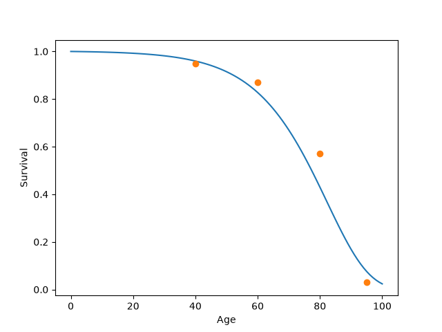
This results in the following life table. Observed values are shown as dots and the line represents the calibrated model.

Bayesian calibration approach

Alternatively, a Bayesian approach can be used to include prior information and parameter uncertainty. PyMC is a Python package for Bayesian inference. Its most efficient samplers are gradient-based. However, the derivative of our log-likelihood function is not available, so those algorithms cannot be used. Instead, our MISCore model can be considered a black box likelihood function and instructions on this page in the PyMC documentation should be followed to use “complex external code” in a PyMC model.

The following code demonstrates how our simple model can be calibrated using PyMC. Following the PyMC tutorials, we write the LogLike class which contains our fit object (our log-likelihood function).

import arviz_plots as azp
import pymc as pm
from pytensor.graph import Apply, Op
import pytensor.tensor as pt

try:
    azp.style.use("arviz-variat")
except ValueError:
    pass


# Our PyTensor Op that integrates our fit object
class LogLike(Op):
    def make_node(self, x) -> Apply:
        x = pt.as_tensor(x)
        inputs = [x]
        outputs = [pt.dscalar()]
        return Apply(self, inputs, outputs)

    def perform(self, node: Apply, inputs: list[np.ndarray], outputs: list[list[None]]):
        # Calculate the log-likelihood by calling our Fit object for these inputs
        loglike_eval = fit(inputs[0])
        outputs[0][0] = np.array([loglike_eval])


loglike_op = LogLike()

with pm.Model():
    # Set prior distributions of the two model parameters
    gompertz_c = pm.LogNormal("gompertz_c", mu=0, sigma=1.5)
    gompertz_scale = pm.LogNormal("gompertz_scale", mu=2, sigma=1)

    # Create custom likelihood function
    x = pm.math.stack([gompertz_c, gompertz_scale])
    pm.Potential("likelihood", loglike_op(x))

    # Calibrate and sample from the posterior distribution
    idata = pm.sample(cores=1, initvals={"gompertz_c": 0.0025, "gompertz_scale": 12})

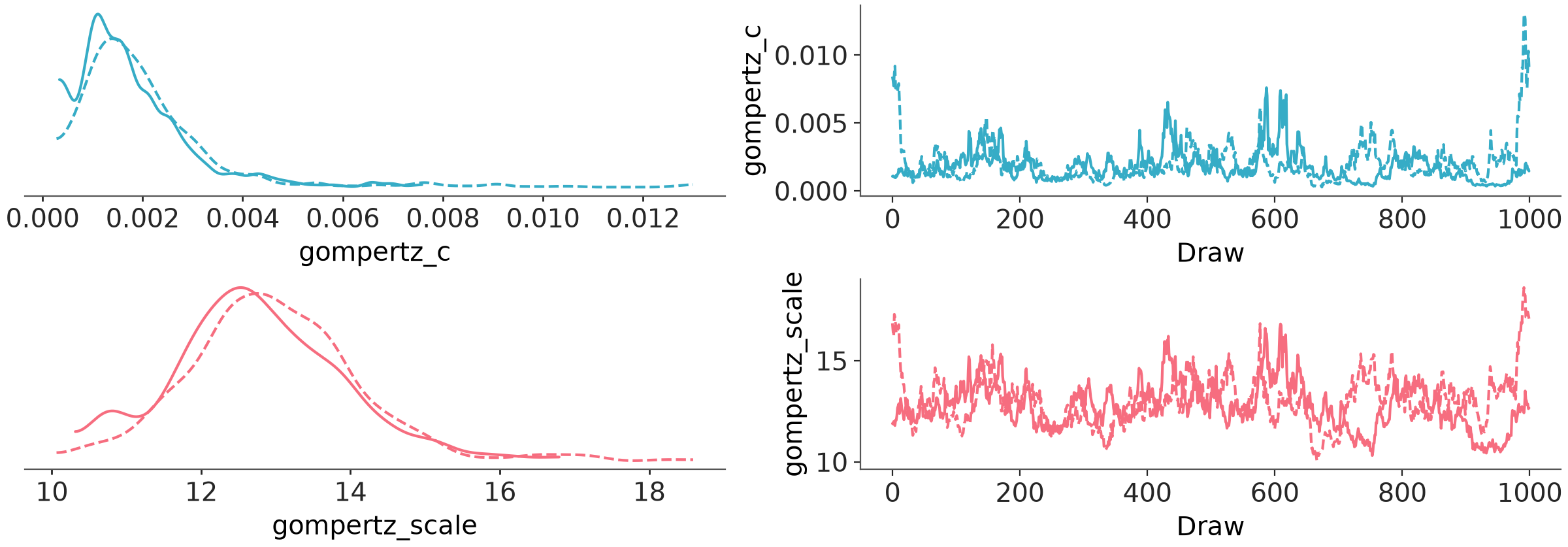
After the calibration, the posterior distribution of the two parameters c and scale can be plotted using ArviZ.

# Plot the posterior distributions of the parameters
azp.plot_trace_dist(idata)
plt.savefig("posterior.png")

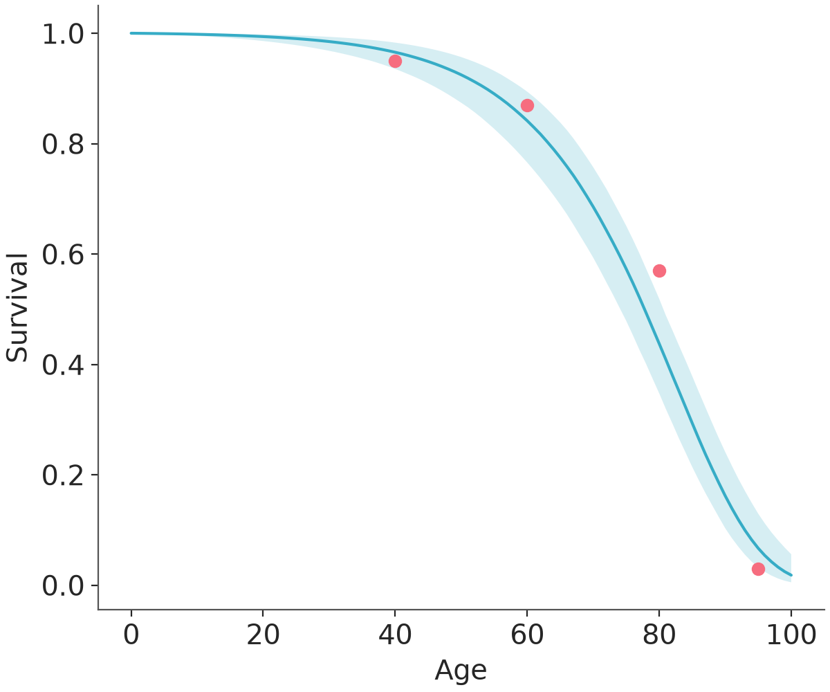
We can also calculate the posterior median and 95% credible interval of our calibrated life table.

# Calculate and plot the posterior median and 95% credible interval of the lifetable
plt.figure()
ages = np.arange(101)
posterior_life_table = stats.gompertz.sf(
    ages[:, None],
    c=idata["posterior"]["gompertz_c"].to_numpy().flatten(),
    scale=idata["posterior"]["gompertz_scale"].to_numpy().flatten()
)
plt.fill_between(
    ages,
    *np.quantile(posterior_life_table, [0.025, 0.975], axis=1),
    alpha=0.2
)
plt.plot(ages, np.quantile(posterior_life_table, 0.5, axis=1))
plt.plot(target_ages[1:], (100 - target.obs.cumsum()[:4]) / 100, "o")
plt.xlabel("Age")
plt.ylabel("Survival")
plt.savefig("life_table_posterior.png")

This results in the following plot. The blue line is the posterior median with 95% credible interval, the dots represent the target data.

A few final thoughts regarding Bayesian calibration:

• This example calibrates a simple model using only a life table. More sophisticated models can be calibrated by modifying the model_from_x() function and specifying the prior distribution of additional parameters, similar to the example in Calibrate a model. Therefore this example can relatively simply be extended to disease models.

• The parameter uncertainty can be propagated to model outcomes by performing model simulations with all samples from the posterior distribution. It is recommended to build a separate Model for each posterior sample, and not to use a separate Universe. Often, the calibrated model parameters are used to generate properties() of a Process and such parameters cannot be varied across universes. See Limits of Universes for further clarification.